This is the fourth piece in a series about building a small language model that writes Magic: The Gathering cards into a compiler I built by hand. The first three pieces got us here: a hand-built compiler that turns Magic’s text into a clean, typed format I can check mechanically, and a hard-won way to keep automated agents honest while they improved it. With all of that in place, I could finally do the thing the whole project was for: train a model to generate that format from plain human intent. This piece is what I found when I did.
One thing before I start. This is not finished research. It is a field journal of an investigation that is still running. It contains results I’m confident in, results that appear to contradict each other, and at least one finding I genuinely cannot fully explain yet. All of it is here, messy parts included, because the messy parts are the real shape of the work.
The ceiling Link to heading
Start with the punchline that sent me looking. I have three models in this project, and I’ll use their project names: dragon (12 billion parameters, a fine-tune of Google’s gemma-4-12b), goblin (4 billion, a fine-tune of gemma-3-4b), and wyrmling (around 110 million parameters, built entirely from scratch: its own architecture, its own tokenizer, no inheritance from anyone). wyrmling also has a 225-million-parameter sibling, same recipe at twice the size, which will matter later. dragon is the best of them. It scores highest on every metric I track.
And it is approaching a wall.
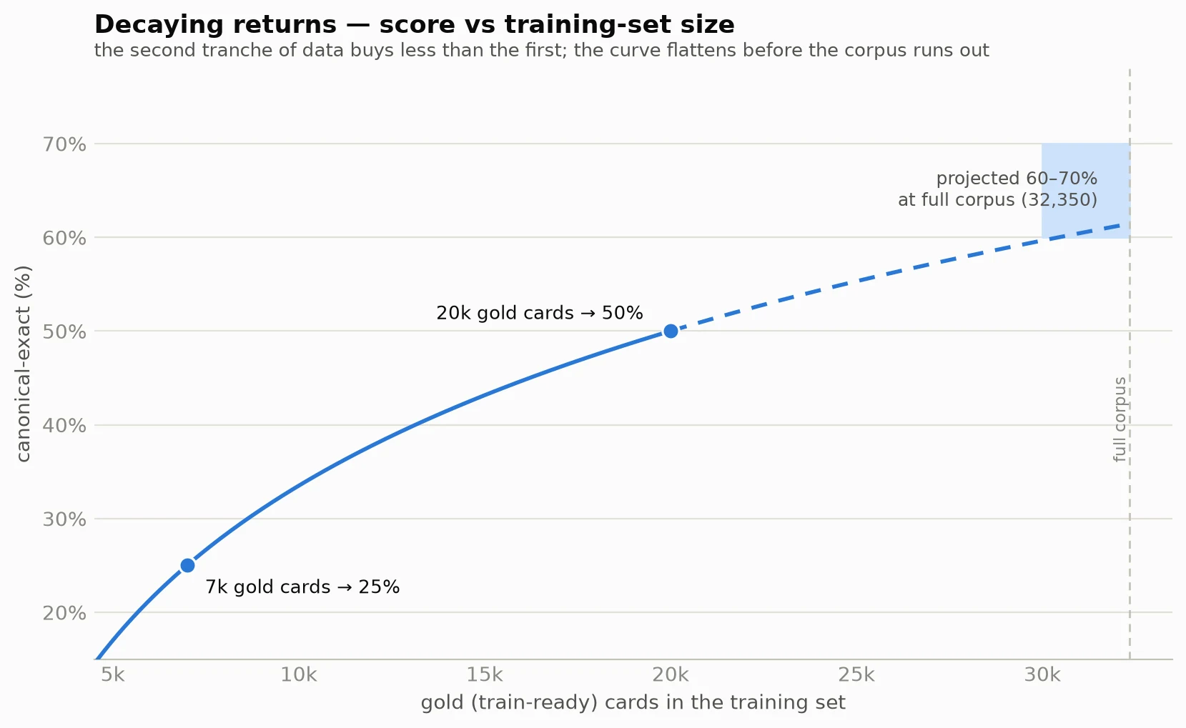
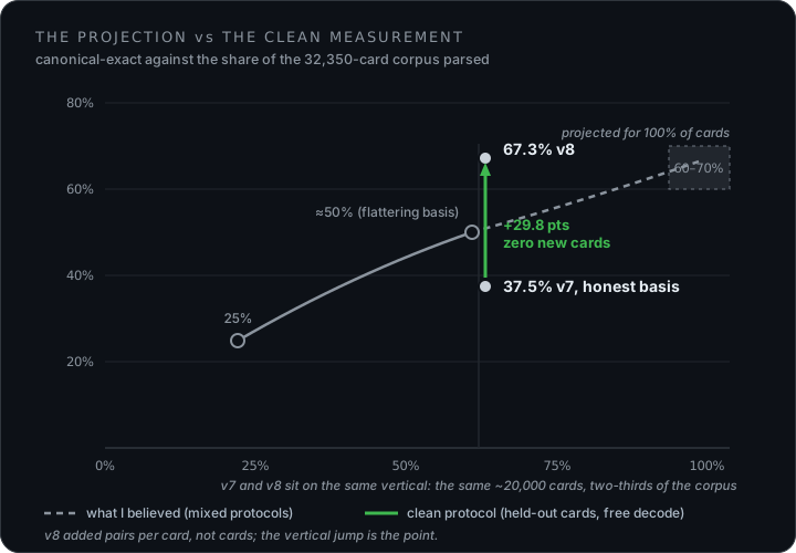
Here’s the subtle part. Dragon keeps improving as I add data; it isn’t frozen. The problem is the shape of that improvement. Early on, with about 7,000 cards in the training set (roughly a fifth of the ~32,000 legal Magic cards), dragon scored around 25%. A fifth of the cards seen, a quarter of them right; nothing alarming. But by my v7 dataset (about 20,000 cards, close to two-thirds of every trainable card in existence) dragon scored around 50%. The ratio doesn’t make sense: I’ve gone from a fifth of the data to two-thirds of the data, and the score only went from a quarter to a half. The return on each new card is decaying. It’s climbing, but the slope is flattening, and it’s running out of raw materials. (One honesty note to hold onto: those two scores come from different eras of my benchmark, under protocols that don’t perfectly match. The shape of the worry was real; hold the exact levels loosely. This piece ends with a cleaner measurement, and it changed my mind about this whole paragraph.)
Because the lever that’s been carrying me is more cards, and there are only roughly 32,000 of them. The only way to get fresh legal cards is to wait months for Wizards to print a new set, which, as the decaying curve already shows, would barely move the needle. My projection is that once I have 100% of the cards in the training set, dragon lands somewhere around 60–70%. (A projection about one lever, more real cards, specifically; keep that in mind, because when dragon does clear 60% at the end of this piece, that is not the lever that did it.) That’s a good number; I want to be clear I’m not calling it a failure. But it’s a long way from perfect, and more importantly, there’s a second problem hiding in plain sight, one that the steady quality gains from each iteration have been quietly masking the whole time.
So this isn’t a post-mortem on a model that hit its ceiling. It’s an ongoing journey I’m going to share: one of the factors I’ve identified for why the scaling isn’t linear, the deceptive results I got along the way, and the luck of having a throwaway experiment hand me a problem that was sitting right in front of my face, one I couldn’t even conceive of until the experiment forced it into view, precisely because my own design choices had hidden it. What you’ll find in this story is about confronting your assumptions, trusting your gut even when the research papers seem to be telling you you’re off track, and the lesson that raw capacity isn’t the only lever, and rarely the one a project this size can afford to reach for. And the thing that taught me all of it was the smallest, least serious model in the project.
The joke that became an instrument Link to heading
wyrmling started as a joke, on my laptop, while I waited.
Fine-tuning dragon takes a long time: multiple days, the kind of wait where you start a run and go find something else to do. During one of those waits, mildly bored, I started building a tiny language model from scratch on my laptop, mostly to see if I still could. I’d built neural networks from scratch before, back in the RNN days, before transformers existed; I wanted to know if I could do it with a modern architecture. There was no serious plan. It was a way to pass the time while the real models trained.
Except there was a little more to it than boredom, and I should be honest about that, because it’s where one of this project’s quieter lessons lives. My gut had been nagging at me about Gemma for a while. It’s a generalist model (it carries capacity for dozens of languages I’ll never touch and abilities I’ll never invoke) and something about pouring my narrow, exotic problem into a model built to do everything felt wrong, like buying a cargo ship to cross a pond. So part of wyrmling was me scratching that itch: what if the right tool for a problem this specialized was something equally specialized, built to do only this?
The trouble was that everything I could find told me the itch was wrong. The literature, the conventional wisdom, and, pointedly, every LLM I asked to help me think it through all pointed the same way: a large pretrained generalist will beat your hand-rolled toy, every time, it’s not close, don’t bother. And here’s the thing I had to sit with, because it’s a lesson that goes beyond this project: that consensus was mostly right, and I still didn’t fully believe it. Not out of stubbornness, out of a habit I’d recommend to anyone. When careful people tell you you’re wrong, the move isn’t to fold, and it isn’t to dig in. It’s to ask why they’re saying it, and to notice that good researchers are scrupulous about marking the border between “this is established” and “this is a reasonable hypothesis given what we know.” The generalist-wins consensus was built on the general case. My case was not general. That gap was narrow, and probably nothing, but it was exactly the kind of gap a throwaway laptop experiment is cheap enough to go poke at.
(There’s a smaller note tucked in here that connects to the previous piece. LLMs are genuinely useful for this kind of thinking: brainstorming, surfacing papers I’d have missed. But they have the same least-friction gravity I watched the coding agents exhibit: ask one whether you should use a battle-tested generalist or build something exotic from scratch, and it will steer you toward the safe, generic, well-trodden answer almost every time. Moving one off that default takes hard evidence, not argument. Keep that in mind whenever you’re using one as a thinking partner: its advice has a bias, and the bias is toward the path of least resistance.)
So I kept tinkering with the joke. And a few things turned it from a way to kill time into the most useful tool in the project.
The first was that I wasn’t the only one with this suspicion. There’s a thread of results in the literature I’d seen and never tested (Fu et al. on specializing smaller models; TinyStories for how far down a narrow domain lets you go): that a small model built for one task can beat a giant generalist at that task, precisely because the giant is spending most of its capacity on everything else. That turned my vague itch into a concrete, testable question: is the giant general pretraining worth more than the capacity I lose by carrying an architecture full of things I don’t need? I genuinely didn’t know, and wyrmling (cheap, fast, disposable) was the perfect way to find out.
And the second thing, the one that actually mattered, was speed. A 110-million-parameter model is so small that I could run a complete cycle, pretraining and fine-tuning, ten or twenty times over in the wall-clock time it took dragon to do a single fine-tune. And a single dragon fine-tune was not quick. I run this on an AMD R9700, a card I chose because it gave me the VRAM I needed for about €2,000 less than the equivalent NVIDIA part. I paid for that saving in other currency: a dragon fine-tune ran about 42 hours in the v7 era and closer to 60 for the v8 run, and getting a clean multi-day run meant fighting ROCm the whole way: out-of-memory failures disguised as inscrutable kernel errors, the server crashing for no reason I could find. The blame for that is entirely mine; I made the price-for-pain trade with my eyes open. But it’s the concrete reason I had so much idle time to fill, and filling it with a laptop-sized model is what turned wyrmling from a toy into a microscope. Experiments that would take weeks to even begin showing a signal on dragon, I could run before lunch on wyrmling. The joke model became the instrument I used to investigate the serious model’s problem, and because it could iterate so fast, it found something the slow, expensive, better model had been hiding.
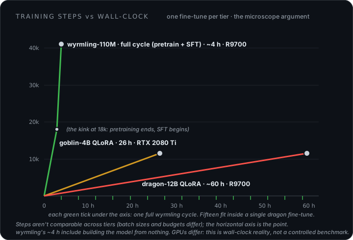
(The microscope argument in one picture: a complete wyrmling cycle, from-scratch pretraining included, fits inside a single dragon fine-tune fifteen times over.)
Shadowing Link to heading
Here is what wyrmling found, and it is the spine of this whole piece.
My DSL describes a Magic card’s abilities. And by the very nature of what it describes, some pieces of it appear in almost every single card. There’s a root node for the card’s abilities. There’s a node marking each individual ability. There are nodes for the things every ability has: what it targets, what it costs, what it does. These structural nodes are everywhere, in card after card after card, because they’re the load-bearing grammar of any ability.
And then there are the rare nodes. Something like a node representing “you win the game” appears on a vanishing handful of cards. It’s a real part of the language (it has to be expressible) but in the actual distribution of Magic cards, it’s a needle in a thirty-thousand-card haystack.
Now think about what happens when you train a model on this. The model learns from the gradient (the correction signal it gets from its mistakes) and that signal is utterly dominated by the nodes that appear constantly. The model sees the structural nodes so many times that it learns them cold. The rare nodes, by contrast, barely register; their signal is drowned out, shadowed, by the overwhelming frequency of the common ones. The model gets excellent at the boilerplate that’s in every card and stays stubbornly bad at the rare effects that make individual cards special, not because those effects are hard, but because they’re outnumbered.
Here is that distribution, measured on the v7 training set, both axes logarithmic, because nothing else can hold it. CREATURE appears 76,284 times. “You win the game” appears 38 times. And 199 node labels appear exactly once in the entire corpus:
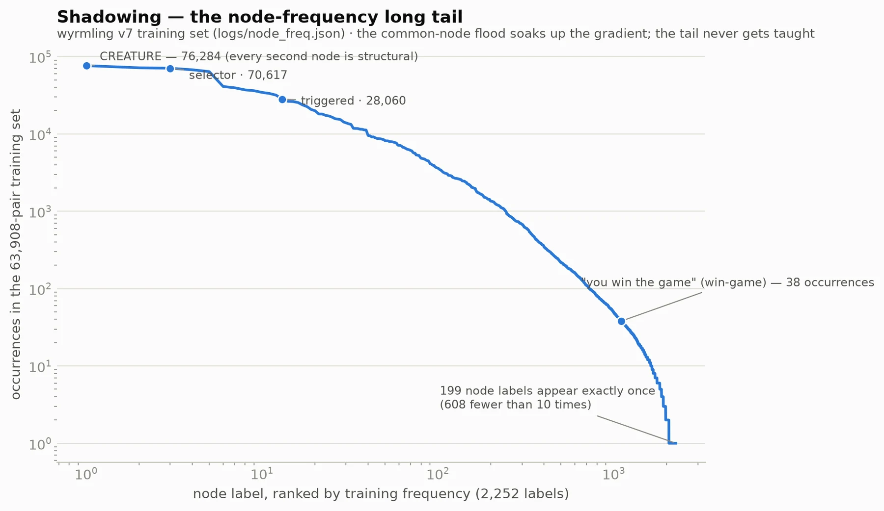
If you’ve written code, you already have the intuition for this. Look at any codebase and count the keywords: you will see def, if, else, for, and while thousands of times, because they’re the basic furniture of the language. You’ll see something like async with far, far less often, because it’s specialized. A model trained on that codebase will produce flawless if/else and fumble the rare constructs, not because they’re conceptually harder, but because it saw them a thousand times less. That’s shadowing. The common drowns the rare, and the rare is often exactly the part you care about.
This is one of the walls all my models were running into, and I’d be surprised if it’s the only one; there may be others I’m not yet aware of. But this one is real, and inside the regime I could actually build and iterate on (small models trained from scratch on this task) it isn’t a capacity problem that more parameters would solve. It’s a distribution problem baked into the training data itself: pile more parameters onto the same shadowed distribution and a small from-scratch model just learns the common nodes a little better while the rare tail stays dark. (Later I’ll put real numbers on that, including the part where a giant pretrained model complicates the story, because the answer surprised me.) Worse, my only lever against it so far has been adding more cards, and once I’ve parsed all of them, that lever is spent. I’ll have maximized my data and still be staring at the shadowed tail. This is exactly where wyrmling’s lack of capacity turned into an asset instead of a handicap: a tiny model was enough to expose the problem, and cheap enough to let me test the fix, fast.
Proving it on a model too small to matter Link to heading
The beauty of having a microscope is that you can run the controlled experiment.
If shadowing is real (if the rare nodes are bad because they’re outnumbered, not because they’re hard) then deliberately changing the training distribution to give the rare nodes more presence should lift them, without needing a bigger model at all. So I tried it on wyrmling. I built a pretraining set that was the natural Magic distribution plus about 18% deliberately “rare-dense” data, over-sampling the shadowed nodes so they’d stop being drowned out, and pretrained wyrmling on it, then fine-tuned exactly as before. The only thing that changed versus the control was the pretraining distribution. Same model size. Same fine-tuning. Same everything else.
The rare tail got better. The nodes that appeared only 10–99 times in the data (the deep shadow) improved their miss rate from 0.709 to 0.638, a 7-point reduction in how often the model got them wrong. The next band up improved too. And critically, the common nodes held: they didn’t degrade to pay for the gain.
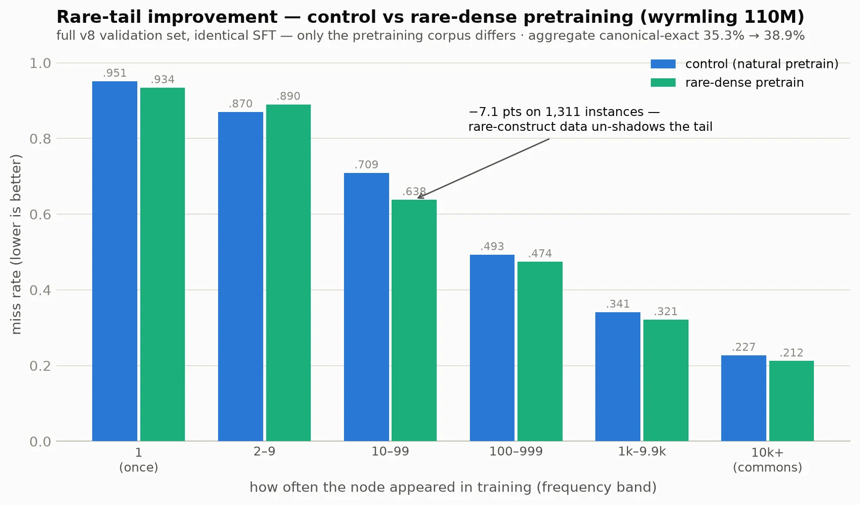
I want to dwell on that last part, because it’s the part I didn’t expect. The intuition you’d bring to this is zero-sum: if you spend more of the model’s attention on rare nodes, surely it comes out of the common ones, and you just move the problem around. That’s not what happened. The rare tail improved, the middle improved, the commons held, and the aggregate scores rose: canonical-exact matches from 35.3% to 38.9%, structural similarity from 0.633 to 0.657. (These absolutes come from the first v8 build, on its validation split, with decoding constrained to the grammar; the cross-tier numbers later in this piece use the rebuilt v8, a held-out test, and free decoding, all of which read higher. Take the shape of the shift here, not the level.) It wasn’t a trade. It was close to a free lunch, bought entirely by changing the shape of the data on a model small enough to fit on a laptop. A 110-million-parameter model un-shadowing its own tail, without scaling anything.
That’s the finding I’m most confident in. The bottleneck dragon kept hitting was never really about dragon. It was shadowing, and for a model the size I could afford to train and re-train, shadowing lives in the data, not the model.
What the scale-up proved, and what it quietly didn’t Link to heading
This is worth pausing on, because it’s the answer to “why build wyrmling at all,” and it surprised me.
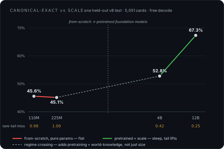
For most of the project I thought I could already see the answer, and I gave it to you a few paragraphs ago: this is the shape of the data, not the size of the model. Then I ran the clean version of the comparison on the v8 dataset (all four models, one held-out test of 5,051 cards, the same free decode, matched generation budgets) and it made me say that far more carefully.
| model | params | parse | canonical-exact | rare-tail miss |
|---|---|---|---|---|
| wyrmling-110M | 118M | 91.6% | 45.6% ±1.4 | 0.98 |
| wyrmling-225M | 226M | 93.1% | 45.1% ±1.4 | 1.00 |
| goblin-4B | 4.3B | 95.6% | 52.8% ±1.4 | 0.42 |
| dragon-12B | 12B | 97.9% | 67.3% ±1.3 | 0.25 |
Read it as two regimes, because that is exactly what it is.
From-scratch, pure parameters: flat. The two wyrmlings are the only genuinely clean size-only comparison in the whole set: same from-scratch recipe, same data, one simply twice the size of the other. Canonical-exact went 45.6% → 45.1%, identical inside the confidence interval, and the shadowed tail, if anything, went a shade darker (the miss rate on the rarest, once-seen nodes drifted 0.98 → 1.00). Doubling a small, data-starved, from-scratch model does nothing for shadowing. That’s the result I built wyrmling to get, and the one I’ll defend hardest.
Foundation scale: steep, and the tail collapses. goblin and dragon tell the opposite story. 52.8%, then 67.3%, each step far outside the interval, and the tail comes back into the light: the miss rate on once-seen nodes falls from ~100% on the wyrmlings to 42% on goblin to 25% on dragon, and the band of nodes seen just two-to-nine times drops from around 0.85 to 0.08. So capacity, at real scale, absolutely can un-shadow the tail. I was about to tell you it couldn’t; as a general law, that would have been wrong.
Here’s the catch that stops me from flipping “data, not size” into “size after all.” That 45→67 climb is not a clean measure of size. wyrmling is from-scratch: the only language it has ever seen is my DSL. goblin and dragon are Gemma foundation models that read a huge slice of the open internet before they ever met a Magic card. So the climb tangles three things at once (more parameters, massive language pretraining, and a world model that already knew what “a +1/+1 counter” is in English), and the one place I can hold pretraining fixed, the two from-scratch wyrmlings, is precisely where scale bought nothing. A 12-billion-parameter model trained from scratch on only my DSL might land nowhere near 67%. I can’t rule it out, because I can’t afford to run it.
And one asterisk on the whole table, which connects straight back to the previous piece: the v8 dataset was cut in late June, a week before the counterfeit-enum burndown landed. Every model here, dragon’s 67.3% included, was trained and evaluated on a language that still carries those 117 fake symbols. The numbers are real, but the language they’re measured on has lead in it; the next dataset is the first one minted after the cleanup, and it’s where the honest version of this table gets to exist.
I even have a guess about who that lead poisons most, and it’s my own optimization biting my hand. wyrmling’s tokenizer is a small one (about twelve thousand tokens) that I trained only on intent-to-DSL pairs, precisely so each DSL concept lands as one semantically loaded token. The counterfeits got that royal treatment too: to wyrmling, a monster like TOTAL_MANA_VALUE_X_OR_LESS_FROM_YOUR_GRAVEYARD is most likely a single opaque token, seen a handful of times in the whole corpus, the purest shadowing bait there is. The Gemma models read the same string through an English tokenizer: to them it’s something like twenty pieces of perfectly ordinary English in a cheap disguise, spaces swapped for underscores, words shouting in caps. The from-scratch models pay full price for every counterfeit; the pretrained ones can partly read their way through the fraud. A guess, not a measurement, but it fits the table above, and it would mean the mint from the last piece taxed exactly the models least able to afford it.
The reason I expected the giant to disappoint is worth keeping, because it turns out to be half right. That giant pretraining is pretraining on human language: understanding English, generating fluent English. But look at what my task actually is. The input the model receives isn’t raw human language at all; by the time it reaches the model, the human’s request has already been parsed into a consistent, structured brief, with no tone or style left to interpret, something like:
Type: Artifact | Colors: W, R | Cost: {1}{W}{R} | Stats: 1/1
Concept: A creature that gains power and toughness when equipped, and
gains deathtouch if it is a Human and equipped. It costs {2} to equip.
And the output isn’t English either; it’s my DSL, a symbolic format I invented, that appears nowhere in any pretraining corpus because it didn’t exist until I made it. For the brief above, what the model is expected to produce looks like this:
(card_abilities
  (static (pt-mod (selector :type CREATURE :states (list EQUIPPED)) +1 +1))
  (static (gain-ability (it) (DEATHTOUCH))
          :condition (is-type :keyword AS :subtype HUMAN :subject-ref EQUIPPED_CREATURE))
  (keyword EQUIP :cost ((mana "{2}"))))
This pair is worth a pause, because it’s a live specimen of what intent-to-DSL training actually has to absorb. The brief is real pipeline output: it was written by gemma-4-e4b (the same mid-sized model behind Verdant Sentinel in the first piece) reading the card’s oracle text, and read closely, it’s nonsense. It declares an Artifact, hands it creature stats, then talks about “a creature that gains power and toughness”, conflating the equipment with the creature wearing it; an artifact can’t be a Human. The target DSL untangles every bit of that: real equipment logic with its {2} equip cost, the boost expressed as a static +1/+1 on the equipped creature, and the deathtouch grant sitting behind a clean condition (the equipped creature being a Human). And the noise is deliberate. Every intent in the dataset is produced by running the full card-generator pipeline on a card’s oracle text (one card, one intent), defects of the generating model included, so that training inputs look exactly like the briefs the model will be handed in production. The job was never pure translation; it’s recovering the structure a confused description was trying to point at.
Neither side of that is English. The input is a rigid structured brief; the output is a symbolic s-expression in a language I made up for a model to generate, all of three months ago. So the model is not really being asked to understand English or write English, the two things all that pretraining is good at. It’s being asked to learn a brand-new symbolic language and translate a rigid brief into it, and that skill comes almost entirely from my fine-tuning data, which is exactly where the shadowing lives.
By that logic the giant’s pretraining should barely help, because I’m hardly using the part of it that’s valuable. And on the clean size-only test, the logic holds perfectly: the two from-scratch wyrmlings are all DSL and no English, and they don’t improve with size at all. What the logic did not predict is dragon. A foundation model doesn’t only carry English; it carries the concepts that English encodes (what a counter is, what an “end step” is, how a condition hangs off an effect), and enough of that apparently survives the jump into a symbolic language I invented to haul the rare tail out of the dark. Whether it’s the scale, the pretraining, or the world-knowledge doing that work, I honestly can’t separate here. What I can isolate is the small-model regime, and there the lever that moved the needle was never parameters. It was the shape of the data, which is exactly why a laptop-sized model was the right instrument to find the problem, and the wrong one to conclude the whole story from.
The contradiction I can’t fully explain Link to heading
Now the part where I keep my promise about the messy bits, because here is a finding that appears to directly contradict everything I just told you about shadowing, and I have not fully resolved it.
Over the life of this project, dragon’s performance roughly doubled, from around 25% to around 50% on my hardest metric (the climb that produced the v7 model, one generation before the v8 numbers in the table above). And the single most reliable way I found to push that number up was to make the DSL more complex: add more node types, handle more cards, enrich the language. Every time I did that, results down the line improved. Consistently. Reliably.
That should not happen. If shadowing is real, then adding more node types means adding more rare nodes: more needles, more things to be shadowed, more dark tail. More complexity should make the shadowing problem worse, and yet more complexity reliably made the results better. I sat with that contradiction for a while, and I still can’t prove which explanation is correct. But here are my guesses.
The most likely explanation, I think, is that two forces are coupled and pulling against each other. In my process, I never added complexity for its own sake; I added it specifically in order to parse more cards, and parsing more cards meant more training data. (I went from about 7,000 cards to about 20,000 over the project’s life.) So every single time I added rare nodes, I simultaneously added a pile of new data. Those two effects are inseparable in how I worked: more rare nodes (which should hurt, via shadowing) always arrived bolted to more data (which helps, via coverage). And it’s entirely possible that, so far, the data-coverage gain has simply been outrunning the added shadowing: shadowing is real and present the whole time, just quietly losing a race against coverage.
If that’s right, it dissolves the contradiction rather than denying it. The production climb couldn’t reveal shadowing cleanly, because every complexity-add confounded “more rare nodes” with “more data”: they moved together, so I could never see their separate effects. wyrmling’s rare-dense experiment could reveal it, precisely because it held the data fixed and changed only the distribution. The two observations aren’t in conflict; they come from experiments that isolate different variables. The microscope saw the thing the production line structurally couldn’t.
I can also rule one thing out, which is its own kind of progress. You might wonder whether the gains came not from the added complexity at all but from a different change: I did, at one point, refactor the DSL to be friendlier for a model to produce (introducing macros, stripping out explicit parameter names), and that refactor alone bought a few points. But that’s not what’s driving this. The clearest evidence is the jump from my v7 dataset to v8: between those two the grammar’s rules held still and the packaging stayed identical; what grew was the node vocabulary (new typed nodes and enums, a slice of which, it turned out, were the counterfeits from the previous piece) and the number of pairs squeezed from each card. The improvement showed up anyway. So whatever is happening, it survives holding the packaging constant. It’s about the complexity-and-data, not the packaging.
Which leaves the honest answer: the coverage-outruns-shadowing hypothesis is my best guess, the format explanation is ruled out, and I have not yet run the controlled experiment that would prove the coverage story rather than merely fit it. So I’m telling you it’s open, because it is.
GCD: the guardrail that made everything worse Link to heading
One more finding, and it’s the one I find most counterintuitive, because it inverts a tool that’s widely treated as a guarantee.
There’s a technique called grammar-constrained decoding (GCD) where you force a model’s output to conform to a formal grammar as it generates, token by token. The model is literally not allowed to produce anything the grammar forbids. It is supposed to be a correctness guarantee: constrain the output, get valid output for free. For a project like mine, where the output has to parse into a strict DSL, GCD sounds like exactly the right insurance.
It made everything worse. On every axis. Including the one it’s supposed to protect.
The speed cost was brutal and almost comic: my DSL grammar is over two thousand lines, and GCD applies the whole thing at every single token, which dropped generation speed by something like 85×. That alone would have been disqualifying. But the genuinely surprising part is that it also made quality worse, the exact thing GCD exists to guarantee.
The reason, once I worked it out, is almost obvious in hindsight, and it ties this whole series together. My DSL was designed for a model to produce. That was the entire point of building it. So models learn it easily: the fine-tuned models produce valid, parseable DSL 95-plus percent of the time without any constraint at all, and even the little from-scratch ones sit above 90%. Which means the grammar constraint wasn’t helping a model that was struggling to produce valid output. It was fighting a model that was already producing valid output, forcing it off the distribution it had comfortably learned and onto the grammar’s rails, and that fight degraded the result. GCD wasn’t insurance. It was a splint on a limb that wasn’t broken, and the splint made the patient walk worse.
But here is the part that matters most, the sentence this whole section exists to deliver. Even when GCD did its job perfectly, even when it forced the output to be valid, parseable DSL, the output still had the wrong semantics, because of shadowing. The model would emit a structurally flawless card that simply didn’t mean the right thing. And GCD is powerless against that, for a reason that is fundamental and not specific to my project: a semantically wrong card can still be a grammatically valid card. GCD enforces form. It cannot enforce content. The shadowing problem lives entirely in the content (in which rare effect the model should have produced) and GCD operates entirely on the form. It was structurally incapable of touching the actual problem. It was, to put it bluntly, a lead bandage: it barely helped, it slowed everything to a crawl, and it could not address the one thing that was actually wrong, because that thing lives in a layer GCD does not reach.
(A tangent from the day job, because the same misconception wears a security costume. If you’re counting on constrained decoding as a defense, “the model can only emit valid JSON, so we’re safe”, think twice. I’ve pentested LLM-powered chatbots and walked XSS payloads out of them inside perfectly valid JSON, because a useful grammar has to allow a free-form string somewhere, and any rule that admits a free string is an injection point the constraint will happily bless. Same story for a constrained SQL grammar that proudly whitelists table names: leave one raw-string position anywhere in it and the whitelist is decoration. GCD buys you form and parse. It does not buy you safety, for exactly the reason it never bought me meaning.)
Where it stands Link to heading
I told you at the top this was a field journal, not a finished result, so let me end where the work actually is rather than tying a bow on it.
The v7 dataset behind dragon’s ~50% had about 70,000 intent-to-DSL training pairs. v8, the set behind the 67.3% in the cross-tier table above, came out after dedup to about 103,000 pairs. And before it does any more quiet work in this piece, I owe you two corrections about what v8 actually is. First: it is not more cards. It’s the same roughly 20,000 gold cards multiplied differently: each gold card spawns rarity-mutated variants, and every variant gets one pipeline-generated intent of its own, exactly the way the original card did. The card-count lever I spent the opening of this piece mourning hasn’t even been pulled. Second: the two numbers I’ve been comparing were never on the same footing. The ~50% I carried around from v7 was the flattering basis; on the honest one (held-out cards, free decoding) dragon-v7 sat at 37.5%. Measured properly on both ends, v7 to v8 took dragon from 37.5% to 67.3%, on a test that is if anything harder than v7’s. That is not a flattening curve politely arriving in the 60–70% band I projected at the start. That’s the projection breaking: the decay I extrapolated was partly an artifact of numbers I should never have compared, and the ~12,000 cards I haven’t parsed yet are still on the table.
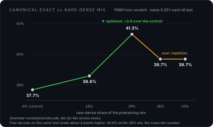
And the rare-dense lever held up at v8 scale, now that the full sweep has run: pretraining mixes at 0, 16, 28, 36 and 43% rare-dense. The optimum moved from the original 18% to 28%, where the 110M model beats its own control on every frequency band, 37.7% to 41.3% canonical-exact under like-for-like decoding (the 45.6% in the cross-tier table is that same model, free-decoded). Past 28% the gains reverse: the finite pool of rare-node samples gets over-repeated. And at 225M the optimum stops being a fixed number and drifts upward, which fits the starvation story; the right mix is a property of the corpus, not the model.
The sweep also quietly handed the contradiction section’s coverage story its first real evidence: the v8 control, with no rare-dense mixing at all, already misses the shadowed 10–99 band far less than the first build’s control did (0.500 versus 0.709). More pairs alone had begun un-shadowing the tail; the deliberate mixing just does it on purpose.
And the next round is already loaded. The v9 dataset is generating as I write this: the first corpus minted since the counterfeit purge (finishing that job had its own twist: on final inspection, two of the three enums I’d spared turned out to be lying too, and only one survived on its merits), and at 442,161 records (20,984 gold cards plus 421,177 mutated variants) it’s roughly five times the v8 training set. Here is what it exists to answer, in the order I care:
- Does retiring rung four’s counterfeit vocabulary move the needle the way the tokenizer story above predicts, now that no model has to waste capacity on 117 fake symbols?
- What do the new transplant mutators buy? They’re a different animal from the rarity tweaks: they operate on the syntax trees themselves, taking valid subtrees from host cards and mixing, grafting, sometimes building cards that never existed. They are fundamentally unsafe from a Magic balance and color-identity standpoint, and the only gate on them is manual human review, so they could optimize the score without optimizing what I actually want from the model. This is the one I’ll be watching with both eyes.
- Does swapping the model that generates the intents cost the intent-to-DSL models quality, or is the intent side cheap to change?
- A mutator-by-mutator audit: every v9 row carries its mutator’s name, so “which mutator earns its keep” becomes a training-time filter instead of a regeneration. Some of them may turn out to inflate the dataset without improving the model trained on it.
- And what this whole table looks like at platinum tier, a quality gate even stricter than the “gold” standard everything above was measured against.
One caveat is already locked in: the v9 held-out split is deliberately harder than v8’s (near-duplicate targets are now purged across splits), so the next round of numbers won’t be directly comparable to this one. Which is, by this point in the project, exactly what I’ve come to expect.
What I do know is the shape of the problem, which is more than I had when I started. The ceiling was never really the model. It was the language: the way a structured DSL, by its own nature, buries its rarest and most interesting pieces under the weight of its most common ones, and how that single property explains why scaling the model I could afford didn’t save me, why changing the data distribution did, and why a grammar that guarantees form can do nothing about meaning. I found all of that with a model small enough to be a joke, because being small made it fast, and being fast made it the only instrument in the project that could actually run the experiments that mattered.
There’s a pattern under all of this that I’ve watched recur through the whole series, and I’ll name it once and leave it. A language model fakes the part of a task it can’t do. An optimizer games the part of a metric you’re measuring. A training distribution drowns the part of a language you most need. A grammar enforces the part of correctness that’s easy and ignores the part that’s hard. Four costumes, one shape: the system pours itself toward whatever signal dominates, and quietly abandons the part that actually matters. Most of the work, it turns out, is noticing where that’s happening, and building the thing that makes the neglected part count.
This is the last of the main pieces. If you want to see the project itself (the compiler, the models, the benchmark, all of it open source) or check where the work stands now, the series hub collects everything.